[Paper Review] Temporal Convolutional Autoencoder for Unsupervised Anomaly Detection in Time Series

논문 링크: Temporal convolutional autoencoder for unsupervised anomaly detection in time series

논문 정보

항목	내용
Venue	Applied Soft Computing
출판 시점	2021년
저자	Markus Thill, Wolfgang Konen, Hao Wang, Thomas Bäck
소속	TH Köln - University of Applied Sciences, Leiden University

핵심 아이디어

TCN-AE(Temporal Convolutional Network Autoencoder) 는 time series anomaly detection을 위한 unsupervised autoencoder이다. 핵심은 fully connected autoencoder나 recurrent model 대신, dilated 1D convolution으로 긴 시간 의존성을 넓은 receptive field에서 학습한다는 점이다.

TCN-AE encoder

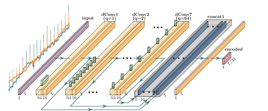
논문 Figure 3. TCN-AE encoder는 ECG signal을 여러 dilation scale의 convolution layer로 처리하고, skip connection으로 각 scale의 feature를 bottleneck에 모은다.

논문이 다루는 문제는 ECG arrhythmia detection이다. ECG anomaly는 한 시점의 값만 이상한 point anomaly가 아니라, 정상적인 peak처럼 보이지만 발생 timing이 어긋나는 collective anomaly일 수 있다. 따라서 local window만 보는 모델은 놓칠 수 있고, 긴 시간 문맥을 보는 모델이 필요하다.

문제 배경

Time series anomaly detection에서는 보통 anomaly label이 부족하다. 그래서 supervised classifier를 학습하기 어렵고, 정상 패턴을 unsupervised 방식으로 학습한 뒤 reconstruction error나 anomaly score로 이상을 판단한다.

ECG anomaly example

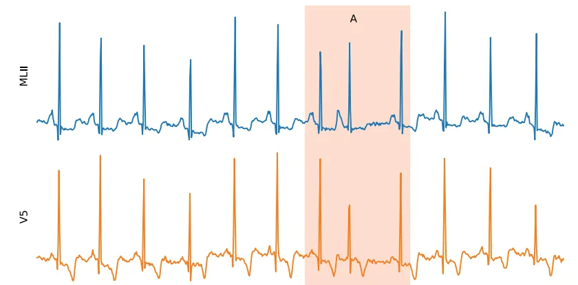
논문 Figure 1. ECG anomaly example이다. Highlight된 영역은 local shape만 보면 정상 peak와 비슷하지만, quasiperiodic pattern 안에서는 timing이 어긋난 anomaly이다.

이 논문의 관점은 다음과 같다.

요구 사항	이유
긴 receptive field	peak가 언제 나와야 하는지 알아야 한다.
multi-scale feature	anomaly가 특정 time scale에서 더 잘 드러날 수 있다.
unsupervised learning	anomaly label이 부족하거나 없는 경우가 많다.
reconstruction 기반 score	정상 pattern을 잘 복원하고 이상 pattern에서 error가 커지도록 한다.

1D Convolution

논문은 먼저 1D convolution을 정의한다. 하나의 time series $x[n]$ 과 finite impulse response filter $h[i]$ 가 있을 때 convolution은 다음과 같다.

y[n] = (x*h)[n] = \sum_{i=0}^{k-1} h[i]\cdot x[n-i]

여기서 $k$ 는 filter length이다. Multivariate time series $x[n]\in\mathbb{R}^d$ 에 대해서는 각 time step의 vector와 filter vector의 dot product로 쓸 수 있다.

y[n] = (x*h)[n] = \sum_{i=0}^{k-1} h[i]^\top x[n-i]

즉 convolution layer는 sliding window 위에서 learnable filter를 적용한다. Time series에서는 이 filter가 특정 temporal pattern을 감지하는 역할을 한다.

Dilated Convolution

TCN-AE의 핵심은 dilated convolution이다. Dilated convolution은 filter tap 사이를 $q$ 만큼 띄운다.

y[n] = (x *_q h)[n] = \sum_{i=0}^{k-1} h[i]^\top x[n-qi]

여기서 $q$ 는 dilation rate이다. $q=1$ 이면 일반 convolution과 같다.

Dilated convolution을 쓰면 parameter 수를 크게 늘리지 않고도 receptive field를 빠르게 키울 수 있다. 예를 들어 dilation rate를

1,2,4,\dots,2^{L-1}

처럼 쌓으면 layer 수 $L$ 에 대해 temporal coverage가 지수적으로 증가한다.

논문은 receptive field를 다음처럼 정리한다.

r_{\text{causal}} = k2^L - 1

r_{\text{acausal}} = \left\lfloor \frac{k}{2}\right\rfloor (2^{L+1}-2)+1

논문에서는 ECG anomaly detection에서 causal convolution과 acausal convolution을 모두 실험했고, 조사한 task에서는 acausal convolution이 조금 더 좋은 결과를 보였다고 설명한다. 다만 acausal convolution은 online setting에서 약간의 delay를 만든다.

Baseline TCN-AE

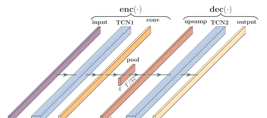
논문 Figure 2. Baseline TCN-AE는 encoder와 decoder로 구성된다. Encoder는 TCN block으로 feature를 압축하고, decoder는 upsampling과 TCN block으로 원래 sequence를 복원한다.

Autoencoder의 기본 목적은 입력 sequence를 압축했다가 다시 복원하는 것이다.

z = \operatorname{enc}(x)

\hat{x} = \operatorname{dec}(z)

학습은 reconstruction loss를 줄이는 방향으로 진행된다. 개념적으로는 다음 objective이다.

\min_{\theta} \sum_n \mathcal{L} \left( x[n], \hat{x}[n] \right)

논문 구현에서는 neural network 학습 loss로 logcosh를 사용한다. 직관적으로 logcosh는 작은 error에 대해서는 MSE처럼 부드럽게 작동하고, 큰 error에는 너무 과도하게 민감해지지 않는다.

Encoder 구조

Encoder는 다음 요소들로 구성된다.

구성 요소	역할
dilated convolution stack	여러 temporal scale의 feature를 추출한다.
`1x1 convolution`	channel 수를 줄여 feature map을 압축한다.
skip connection	각 dilation scale의 feature를 bottleneck 쪽으로 전달한다.
average pooling	time axis를 downsample하여 compressed representation을 만든다.

논문에서 최종 TCN-AE는 encoder에 7개의 dilated convolution layer를 둔다. Dilation rate는 다음과 같다.

q_{\text{enc}} = (1,2,4,\dots,64)

각 dilated convolution layer의 출력은 1x1 convolution으로 channel 수가 줄어든 뒤 concat된다. 논문 설정에서는 각 layer에서 16 channel로 줄이고, 7개 layer를 concat하므로

7 \cdot 16 = 112

channel이 bottleneck 전에 모인다.

TCN-AE는 마지막 layer feature만 쓰지 않고, 여러 dilation scale의 hidden representation을 함께 사용한다.

Decoder 구조

TCN-AE decoder

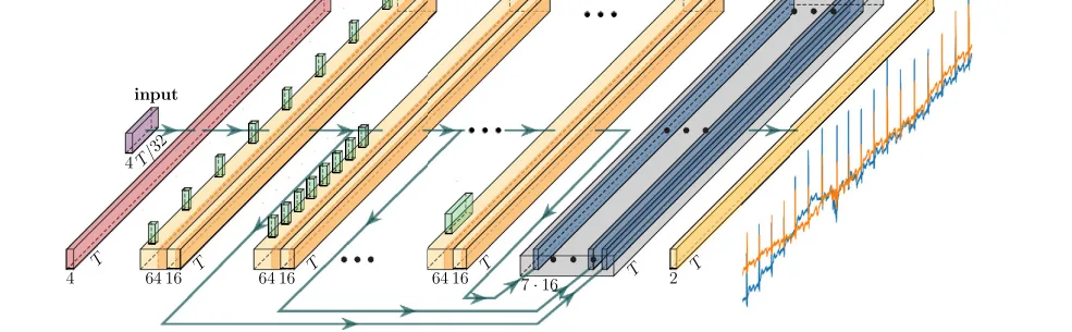
논문 Figure 4. Decoder는 compressed representation을 upsampling한 뒤, dilated convolution stack과 skip connection을 통해 원래 ECG sequence를 복원한다.

Decoder에서도 dilated convolution stack을 사용한다. 다만 dilation rate 순서를 encoder와 반대로 둔다.

q_{\text{dec}} = (64,32,16,\dots,1)

이 선택은 upsampling 직후의 coarse signal에서 큰 dilation을 먼저 쓰고, output에 가까워질수록 작은 dilation으로 detail을 복원하려는 설계이다.

마지막에는 linear activation을 가진 convolution layer가 원래 ECG dimension으로 sequence를 복원한다.

Anomaly Score

TCN-AE는 reconstruction error를 anomaly signal로 사용한다. 입력과 복원값이

x[n], \quad \hat{x}[n]

일 때 reconstruction error를 단순화하면 다음처럼 볼 수 있다.

e[n] = x[n]-\hat{x}[n]

하지만 논문은 단순히 $|e[n]|$ 하나만 thresholding하지 않는다. Reconstruction error 위에 길이 $\ell$ 의 sliding window를 적용하여 error matrix를 만든다.

E[n] = \begin{bmatrix} e[n-\ell+1] \\ \vdots \\ e[n] \end{bmatrix}

여기에 encoder의 hidden representation에서 나온 추가 signal도 stack한다. 논문 설정에서는 reconstruction error가 2-dimensional ECG signal이고, encoder의 7개 dilated layer output을 추가로 사용하여 총 9-dimensional signal을 anomaly detection에 사용한다.

마지막 anomaly score는 Mahalanobis distance로 계산한다.

M[n] = (E'[n]-\mu)^\top \Sigma^{-1} (E'[n]-\mu)

여기서 $\mu$ 와 $\Sigma$ 는 error vector의 mean과 covariance matrix이다. 이 score가 threshold보다 크면 anomaly로 판단한다.

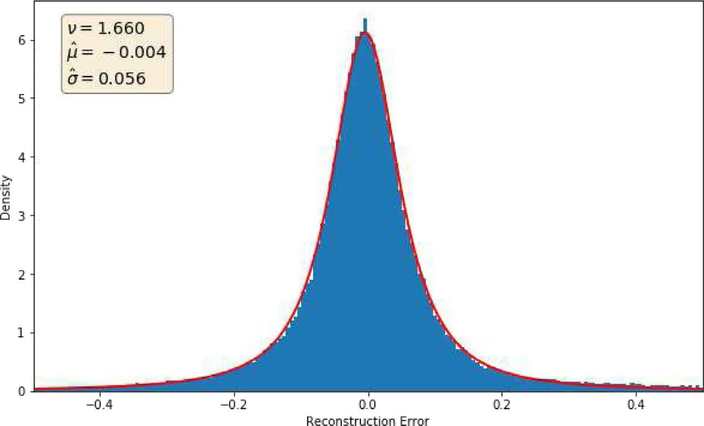
Reconstruction error distribution

논문 Figure A.12. Reconstruction error distribution 예시이다. 논문은 error vector에 대해 Mahalanobis distance를 적용해 anomaly score를 만든다.

전체 Algorithm

논문의 anomaly detection pipeline은 다음처럼 정리할 수 있다.

ECG time series를 정규화한다.
Sliding window로 training sample을 만든다.
TCN-AE를 unsupervised 방식으로 학습한다.
입력 $x[n]$ 을 복원하여 $\hat{x}[n]$ 을 얻는다.
Reconstruction error와 hidden representation signal을 stack한다.
Error window $E'[n]$ 를 만든다.
Mahalanobis distance $M[n]$ 를 anomaly score로 계산한다.
Threshold를 넘는 구간을 anomaly로 판단한다.

중요한 점은 TCN-AE 학습 자체에는 anomaly label이 들어가지 않는다는 것이다. 논문은 threshold 선택에는 일부 label을 쓰는 setting도 비교하지만, model training은 unsupervised이다.

실험 설정

논문은 MIT-BIH Arrhythmia benchmark를 사용한다. ECG signal은 두 channel로 구성된다.

항목	내용
Dataset	MIT-BIH Arrhythmia database
Signal	MLII와 modified lead V1
Sampling frequency	360 Hz
Recording length	약 30분
사용한 time series	25개 ECG recording
anomaly class	9개 anomaly type

비교 대상은 DNN-AE, LSTM-ED, LSTM-AD, NuPIC, LOF, GMM, BGMM, Isolation Forest, OCC-SVM, SORAD 등이다.

평가 지표는 precision, recall, $F_1$ score이다.

\operatorname{Prec} = \frac{TP}{TP+FP}

\operatorname{Rec} = \frac{TP}{TP+FN}

F_1 = 2\cdot \frac{\operatorname{Prec}\cdot \operatorname{Rec}} {\operatorname{Prec}+\operatorname{Rec}}

실험 결과

Precision recall curve

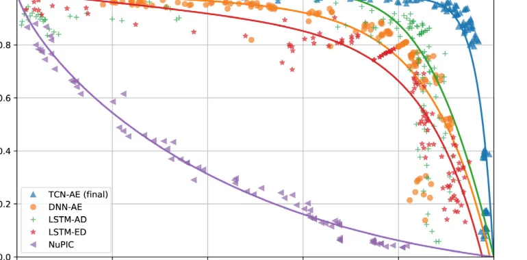
논문 Figure 8. Deep learning 기반 anomaly detection 방법들의 precision-recall curve이다. TCN-AE final이 높은 precision을 유지한 채 recall을 크게 가져간다.

논문의 주요 결과는 다음과 같다.

Model	Precision	Recall	$F_1$
`TCN-AE final`	0.923	0.930	0.926
`TCN-AE baseline`	0.822	0.829	0.826
`LSTM-AD`	0.812	0.817	0.815
`DNN-AE`	0.803	0.810	0.806
`LSTM-ED`	0.767	0.773	0.770
`NuPIC`	0.311	0.311	0.311

TCN-AE final은 baseline보다 약 0.10 높은 $F_1$ score를 보인다. 논문은 skip connection, hidden representation 활용, decoder dilation 순서 반전, anomaly score baseline correction 등이 모두 성능 향상에 기여한다고 분석한다.

특히 skip connection을 제거하면 $F_1$ 이 약 0.93에서 약 0.86으로 떨어진다. 이는 여러 time scale의 feature reuse가 이 architecture에서 중요하다는 점을 보여준다.

장점

Dilated convolution으로 long-range temporal pattern을 효율적으로 본다.
Autoencoder 구조라 anomaly label 없이 학습할 수 있다.
여러 dilation scale의 hidden representation을 anomaly score에 활용한다.
Decoder dilation rate를 반대로 배치하여 coarse-to-fine reconstruction을 유도한다.
ECG benchmark에서 기존 unsupervised anomaly detection 방법보다 높은 성능을 보인다.

한계

TCN-AE는 대부분의 data가 normal behavior라는 가정에 의존한다. 논문도 anomaly가 너무 많은 time series에서는 성능이 무너질 수 있다고 설명한다. Autoencoder가 anomaly까지 정상적으로 복원해버리면 reconstruction error 기반 detection은 약해진다.

또한 threshold 선택 문제는 완전히 사라지지 않는다. Mahalanobis distance로 score를 만들더라도, 실제 운영에서는 threshold를 어떻게 정할지가 여전히 중요하다.

마지막으로 acausal convolution은 offline 분석에서는 유리하지만, online detection에서는 delay를 만들 수 있다. 실시간 system에서는 causal model과 성능 trade-off를 다시 봐야 한다.

정리

TCN-AE는 time series anomaly detection에서 중요한 사실을 잘 보여준다.

이상은 한 시점의 값이 아니라, 시간적 문맥과 multi-scale pattern 안에서 정의될 수 있다.

이 논문의 핵심은 TCN을 단순 forecasting model로 쓰지 않고, dilated convolution 기반 autoencoder로 정상 sequence의 multi-scale 구조를 학습한다는 점이다. 그리고 reconstruction error만 보지 않고 hidden representation까지 anomaly score에 넣어, 여러 time scale에서 anomaly를 찾는다.