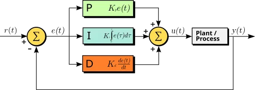
PID (Proportional Integral Differential)는 피드백 기반 제어 알고리즘이다.
이 알고리즘은 목표값(setpoint, SP)과 실제값(process variable, PV)의 차이를 비교한다.
이 차이를 에러값, $e(t)$ 라고 표현한다.

pid-controller-wikipedia
출처: Wikipedia: Proportional-integral-derivative controller

3가지 제어로 나누어져 있다.

비례(Proportional)
적분(Integral)
미분(Derivative)

pid-parameter-plot

1. Proportional Control

비례 제어(Proportional Control) 는 목표값과 실제값 간의 '현재 오차(Error)'에 비례하여 제어량을 결정한다.

핵심 원리: 오차가 크면 제어량을 크게 하고, 오차가 작으면 제어량을 작게 만든다.
비유: 자동차 운전 시 차선 중앙에서 많이 벗어났을 때 핸들을 크게 꺾고, 조금 벗어났을 때 작게 꺾는 것 같다.
장점: 구현이 간단하고 시스템에 즉각적으로 반응하여 오차를 빠르게 줄일 수 있다.

2. Integral Control

적분 제어(Integral Control) 는 시간에 따라 누적된 '과거의 오차'를 바탕으로 제어량을 결정한다.

핵심 원리: 비례 제어만으로 해결되지 않는 작은 정상상태 오차가 계속 쌓이면, 이 누적된 값을 기반으로 제어량을 점차 키워 오차를 완전히 제거한다.
비유: 샤워기 온도를 맞출 때, 물이 계속 미지근하면 아주 조금씩 뜨거운 물 쪽으로 손잡이를 계속 돌려 원하는 온도를 정확히 맞추는 것과 같다.
장점: 비례 제어의 한계인 정상상태 오차를 효과적으로 제거하여 제어의 정밀도를 높인다.

3. Derivative Control

미분 제어(Derivative Control) 는 오차의 변화율, 즉 오차가 얼마나 빠르게 변하는지를 감지하여 '미래의 오차'를 예측하고 이에 대응한다.

핵심 원리: 오차가 목표값을 향해 급격하게 줄어들고 있다면, 목표값을 지나쳐버릴 것을 예측하고 미리 제어량을 줄여 '브레이크'를 걸어준다. 이를 통해 오버슈트를 억제하고 안정성을 높인다.
비유: 목적지에 빠르게 접근하는 자동차가 정지선을 지나치지 않도록 미리 속도를 줄이는 것과 같다.
장점: 오버슈트를 줄이고 목표값에 더 빨리 안정적으로 수렴하도록 도와 시스템의 반응 속도와 안정성을 향상시킨다.

수학적 해석

Control function

u(t) = K_p e(t) + K_i \int_{0}^{t} e(\tau)d\tau + K_d \frac{de(t)}{dt}

$u(t)$ : 시간 $t$ 에서의 최종 제어 출력값
$e(t)$ : 시간 $t$ 에서의 오차(Error). 목표값(SP) - 현재값(PV)로 계산
$K_p$ , $K_i$ , $K_d$ : 각각 비례, 적분, 미분 항의 이득(Gain).
$t$ : 현재 시간

Standard form

위 Control function에서 $K_p$ 를 괄호 밖으로 묶어내고, 적분 및 미분 동작을 시간 상수( $T_i$ , $T_d$ )로 표현한다.

u(t) = K_p \left( e(t) + \frac{1}{T_i} \int_{0}^{t} e(\tau)d\tau + T_d\frac{de(t)}{dt} \right)

$K_p$ : 비례 이득(Proportional Gain). 제어기 전체의 반응 강도를 조절하는 기본 Gain이다.
$T_i$ : 적분 시간(Integral Time). 적분항이 비례향만큼 제어 출력을 만드는 데 걸리는 시간이다. 이 값이 작을수록 적분 제어 영향력이 강해져 정상상태 오차를 더 빠르게 제거한다.
$T_d$ : 미분 시간(Derivative Time). 미분항이 미래의 오차를 예측하는 시간을 의미한다. 이 값이 클 수록 미분 제어 영향력이 강해져 시스템의 진동을 더 효과적으로 억제한다.

T_i = \frac{K_p}{K_i}

T_d = \frac{K_d}{K_p}

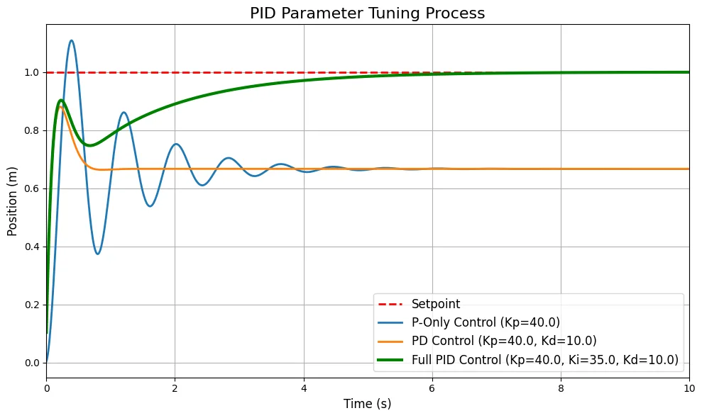
Mass Spring Damper 예제

import matplotlib.pyplot as plt
import numpy as np


Kp = 40.0  # Proportional Gain
Ki = 35.0  # Integral Gain
Kd = 10.0  # Derivative Gain

# System: Mass-Spring-Damper
m = 1.0  # Mass (kg)
k = 20.0 # Spring constant (N/m)
c = 2.0  # Damping coefficient (Ns/m)

# Simulation Parameters
dt = 0.01
total_time = 10.0
steps = int(total_time / dt)
setpoint = 1.0


def run_simulation(gains, system_params):
    kp, ki, kd = gains
    m, k, c = system_params

    # Initialize state
    y = 0.0
    y_dot = 0.0
    integral = 0.0
    prev_err = 0.0

    # Data log
    y_history = []

    for _ in range(steps):
        # 1. Calculate Error
        err = setpoint - y

        # 2. Calculate Integral and Derivative terms
        integral += err * dt
        derivative = (err - prev_err) / dt

        # 3. Calculate PID Control Input (u)
        u = kp * err + ki * integral + kd * derivative
        prev_err = err

        # 4. Update System Model based on physics
        # m*a + c*v + k*x = u  =>  a = (u - c*v - k*x) / m
        y_ddot = (u - c * y_dot - k * y) / m  # Acceleration
        y_dot += y_ddot * dt                  # Velocity
        y += y_dot * dt                       # Position

        y_history.append(y)

    return y_history


y_p_only = run_simulation((Kp, 0, 0), (m, k, c))

# Run PD simulation
y_pd = run_simulation((Kp, 0, Kd), (m, k, c))

# Run full PID simulation
y_pid = run_simulation((Kp, Ki, Kd), (m, k, c))

# Time vector for plotting
t_his = np.arange(0, total_time, dt)

plt.figure(figsize=(10, 6))
plt.plot(t_his, [setpoint] * steps, 'r--', linewidth=2, label='Setpoint')
plt.plot(t_his, y_p_only, linewidth=2, label=f'P-Only Control (Kp={Kp})')
plt.plot(t_his, y_pd, linewidth=2, label=f'PD Control (Kp={Kp}, Kd={Kd})')
plt.plot(t_his, y_pid, 'g-', linewidth=3, label=f'Full PID Control (Kp={Kp}, Ki={Ki}, Kd={Kd})')

plt.title('PID Parameter Tuning Process', fontsize=16)
plt.xlabel('Time (s)', fontsize=12)
plt.ylabel('Position (m)', fontsize=12)
plt.grid(True)
plt.legend(fontsize=12)
plt.xlim(0, total_time)
plt.tight_layout()
plt.show()

PID Control System