[Machine Learning] Edge Detection with Python

Sobel 알고리즘은 영상 처리에서 엣지 검출을 위해 사용하는 필터로, 이미지의 각 픽셀에서 그래디언트(gradient)를 계산하여 엣지를 감지한다.

이 알고리즘은 두 개의 방향(수직과 수평)의 그래디언트를 계산하기 위해 Sobel 커널을 사용한다.

Sobel 필터

Sobel 필터는 수직 방향과 수평 방향을 계산하기 위한 두 개의 3×3 커널로 구성된다.

수직 방향 Sobel 필터 (G_x):

G_x = \begin{bmatrix} -1 & 0 & 1 \\ -2 & 0 & 2 \\ -1 & 0 & 1 \end{bmatrix}

수평 방향 Sobel 필터 (G_y):

G_y = \begin{bmatrix} -1 & -2 & -1 \\ 0 & 0 & 0 \\ 1 & 2 & 1 \end{bmatrix}

Sobel 알고리즘

그레이스케일 변환

입력 이미지를 그레이스케일로 변환하여 단일 채널 이미지를 얻는다. 이를 통해 계산량을 줄이고, 밝기 정보만으로 엣지를 감지한다.

그레이스케일 변환은 다음 식을 사용한다:

I_{\text{gray}}(x, y) = 0.299R(x, y) + 0.587G(x, y) + 0.114B(x, y)

그래디언트 계산

수직 방향(G_x)과 수평 방향 (G_y)의 그래디언트를 Sobel 필터와의 합성곱(convolution)을 통해 계산한다. 합성곱은 다음 식으로 표현된다:

G_x(x, y) = \sum_{i=-1}^{1} \sum_{j=-1}^{1} G_x[i, j] \cdot I_{\text{gray}}(x+i, y+j)

G_y(x, y) = \sum_{i=-1}^{1} \sum_{j=-1}^{1} G_y[i, j] \cdot I_{\text{gray}}(x+i, y+j)

그래디언트 크기 계산

두 방향의 그래디언트 값을 결합하여 최종 엣지 강도를 계산한다. 그래디언트 크기는 다음 식으로 계산한다:

G(x, y) = \sqrt{G_x^2(x, y) + G_y^2(x, y)}

시각화

계산된 그래디언트 크기 G(x, y)는 엣지 강도를 나타내는 값으로, 이를 이용해 깊이 맵을 생성하거나 시각화한다.

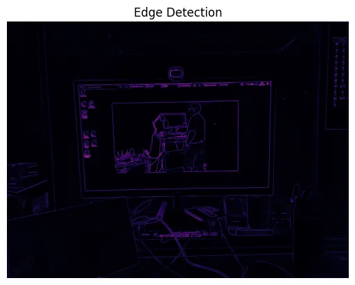
문제점 발생

위 Sobel 알고리즘으로 다음과 같이 경계선 탐지(Edge Detection)과는 거리가 먼 결과물이 나왔다. 몇 번 검색해보니 멀티 스케일(Multi-scale) 작업을 해줘야 했다.

Multi Scale

멀티 스케일(Multi-scale)은 복잡한 시스템이나 데이터를 여러 스케일(크기나 해상도)에서 분석하고 처리하는 알고리즘이다.

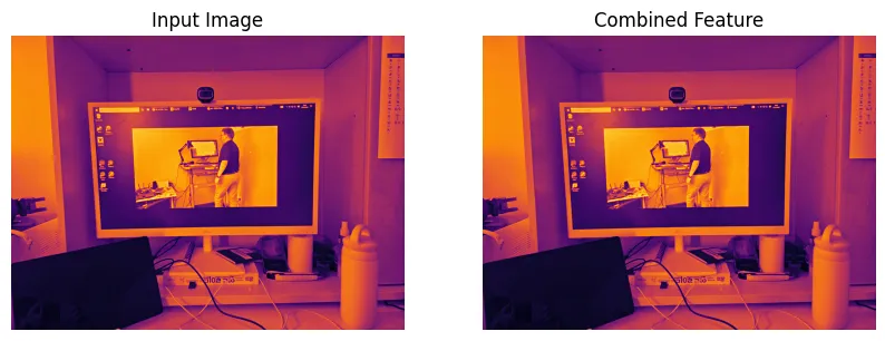
간단히 원본, 1/2 배, 1/4 배 이미지를 합쳐서 사용한다. 이미지가 원본에 가까울 수록 이미지의 형태를 잘 해석하고, 이미지가 작아질 수록 이미지의 경계를 잘 해석하는 경향이 있다.

필자는 다음과 같이 구현해보았다:

import numpy as np
import matplotlib.pyplot as plt
import cv2

# Load input image (example image used)
image_height, image_width = 100, 100

# Convert to Grayscale
gray_image = cv2.imread('./data/test.png', 0)  # Load image in grayscale mode

# Multi-Scale Feature Extraction
def downsample(image, scale):
    """
    Reduce the size of an image by the given scale factor

    Args:
        image (numpy.ndarray): The input image
        scale (int): The scale factor

    Returns:
        numpy.ndarray: The downsampled image
    """
    h, w = image.shape
    new_h, new_w = h // scale, w // scale
    return image[::scale, ::scale]

def upsample(image, original_shape):
    """
    Enlarge an image to match the original shape

    Args:
        image (numpy.ndarray): The input image
        original_shape (tuple): The original shape of the image

    Returns:
        numpy.ndarray: The upsampled image
    """
    scale_h = original_shape[0] // image.shape[0]
    scale_w = original_shape[1] // image.shape[1]
    return np.repeat(np.repeat(image, scale_h, axis=0), scale_w, axis=1)

# Define scales for multi-scale features
scales = [1, 2, 4]
multi_scale_features = [gray_image] + [downsample(gray_image, scale) for scale in scales]

Multi Scale 적용 전

멀티 스케일(Multi-scale)을 적용하기 전 즉, 원본 이미지만 넣었을 때 다음과 같이 경계선 탐지(Edge Detection)가 잘 안되는 모습이다.

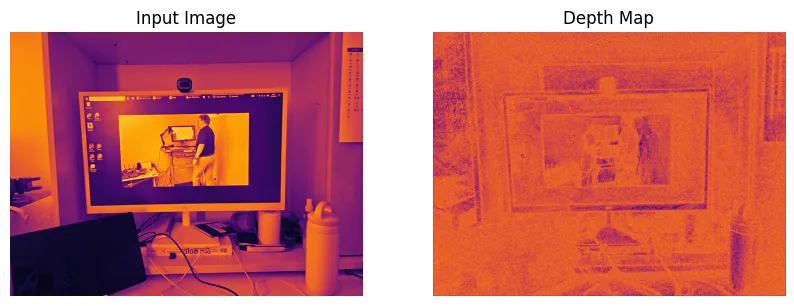
Multi Scale 적용 후

원본 이미지/멀티 스케일(Multi-scale) 이미지
멀티 스케일(Multi-scale) 이미지는 원본 이미지보다 화질이 떨어져보이지만, 경계선이 전보다 확실히 구분된다.

결과물

import numpy as np
import matplotlib.pyplot as plt
import cv2

# Load input image (example image used)
image_height, image_width = 100, 100

# 1. Convert to Grayscale
gray_image = cv2.imread('./data/test2.png', 0)  # Load image in grayscale mode

# 2. Multi-Scale Feature Extraction

def downsample(image, scale):
    """Reduces the size of an image by the given scale factor.

    Args:
        image (ndarray): Input image.
        scale (int): Scale factor for downsampling.

    Returns:
        ndarray: Downsampled image.
    """
    h, w = image.shape
    new_h, new_w = h // scale, w // scale
    return image[::scale, ::scale]

def upsample(image, original_shape):
    """Enlarges an image to match the original shape.

    Args:
        image (ndarray): Input image.
        original_shape (tuple): Shape to upsample to (height, width).

    Returns:
        ndarray: Upsampled image.
    """
    scale_h = original_shape[0] // image.shape[0]
    scale_w = original_shape[1] // image.shape[1]
    return np.repeat(np.repeat(image, scale_h, axis=0), scale_w, axis=1)

# Define scales for multi-scale features
scales = [1, 2, 4]
multi_scale_features = [gray_image] + [downsample(gray_image, scale) for scale in scales]

# Initialize combined feature map with float64 type
combined_feature = np.zeros_like(gray_image, dtype=np.float64)

# Combine multi-scale features
for feature in multi_scale_features:
    if feature.shape != gray_image.shape:
        # Upsample smaller-scale images to match original image size
        feature = upsample(feature, gray_image.shape)
    combined_feature += feature

# Normalize the combined feature map after float operations
combined_feature /= len(multi_scale_features)

# Visualize results
plt.figure(figsize=(10, 5))

# Display the input grayscale image
plt.subplot(1, 2, 1)
plt.title("Input Image")
plt.imshow(gray_image, cmap="inferno")
plt.axis("off")

# Display the combined feature map
plt.subplot(1, 2, 2)
plt.title("Combined Feature")
plt.imshow(combined_feature, cmap="inferno")
plt.axis("off")

plt.show()

# 4. Sobel Edge Detection (Simple depth cue)
sobel_x = np.array([[-1, 0, 1], [-2, 0, 2], [-1, 0, 1]])  # X-direction filter
sobel_y = np.array([[-1, -2, -1], [0, 0, 0], [1, 2, 1]])  # Y-direction filter

# Initialize gradient maps for X and Y directions
depth_x = np.zeros_like(combined_feature)
depth_y = np.zeros_like(combined_feature)

# Apply Sobel filters to calculate gradients
for i in range(1, combined_feature.shape[0] - 1):
    for j in range(1, combined_feature.shape[1] - 1):
        region = combined_feature[i-1:i+2, j-1:j+2]  # Extract 3x3 region
        depth_x[i, j] = np.sum(region * sobel_x)  # Convolve with Sobel X
        depth_y[i, j] = np.sum(region * sobel_y)  # Convolve with Sobel Y

# Compute final depth map as the magnitude of gradients
depth_map = np.sqrt(depth_x**2 + depth_y**2)

# 5. Normalize depth map to range 0-1
depth_map = (depth_map - depth_map.min()) / (depth_map.max() - depth_map.min())

# Visualize results
plt.title("Edge Detection")
plt.imshow(depth_map, cmap="inferno")
plt.axis("off")
plt.show()